In this chapter, we will explore the key properties of Principal Component Analysis (PCA). These properties are essential to understanding how PCA works, how much information is retained after dimensionality reduction, and how the original data can be reconstructed from the principal components.
5.1 Explained Variance
One of the core properties of PCA is its ability to maximize variance in the data. The principal components are ordered such that the first principal component captures the largest possible variance, and each succeeding component captures the maximum remaining variance under the constraint that it is orthogonal to the previous components.
5.1.1 Definition of Explained Variance
The explained variance of the \(i\)-th principal component is the amount of variance in the data that is captured by that component. The total variance in the data is the sum of all the variances along the principal components (the eigenvalues).
Let \(\lambda_i\) represent the eigenvalue corresponding to the \(i\)-th principal component. The explained variance of the \(i\)-th principal component is:
\[
\text{Explained Variance}_i = \lambda_i
\]
The total variance in the data is the sum of all eigenvalues:
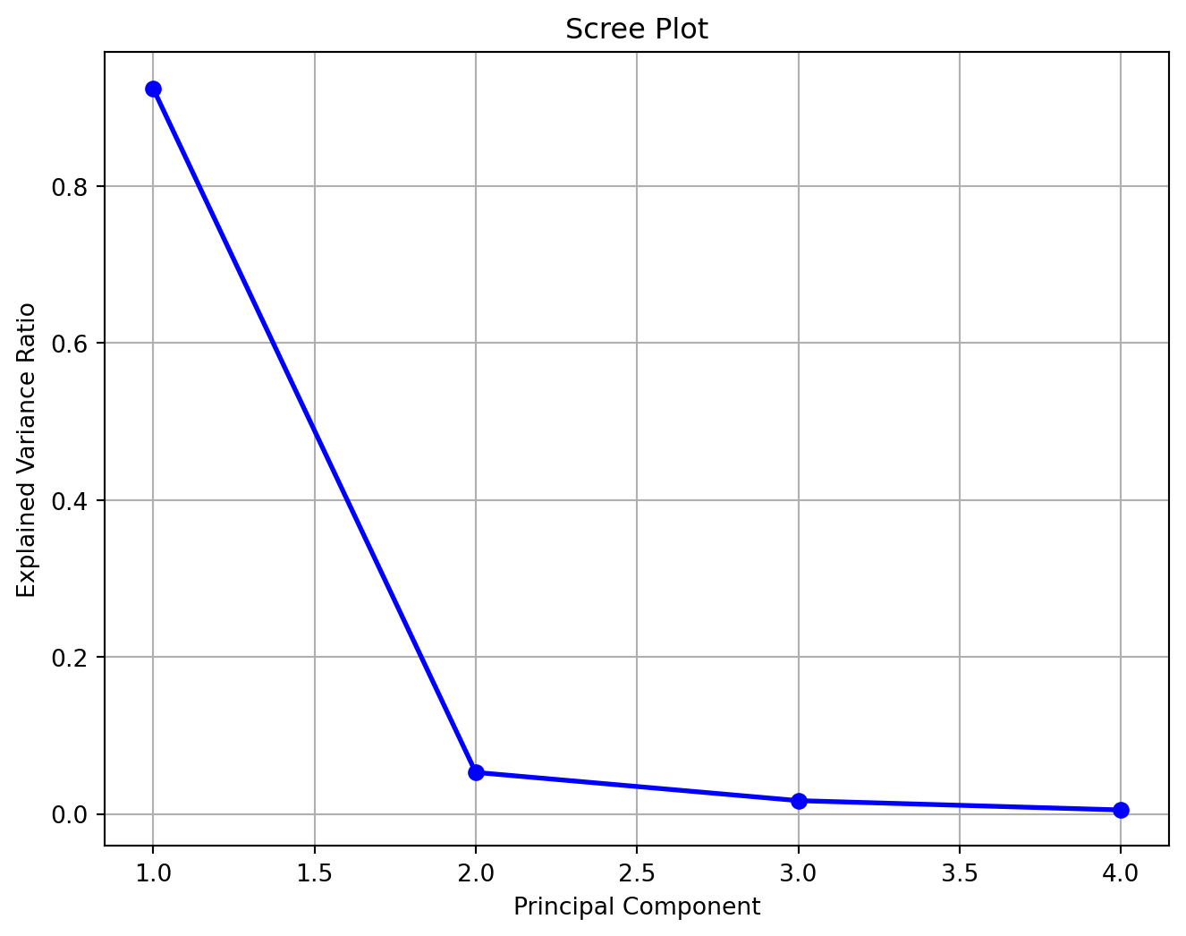
A Scree Plot is a visual tool used to show the eigenvalues (or explained variance ratios) in descending order. It helps in determining the number of principal components to retain.
The x-axis of the Scree Plot shows the number of principal components.
The y-axis shows the corresponding eigenvalues or explained variance ratios.
A “knee” in the plot, where the eigenvalues start to level off, indicates that most of the important variance is captured by the components to the left of the knee.
Example 5.1 (Example: Scree Plot) Below is an example Python code for generating a Scree Plot using the Iris dataset and PCA:
In this example, the Scree Plot helps you decide how many components to retain by looking for the “elbow” or “knee” in the curve.
5.2 Dimensionality Reduction
PCA is commonly used for dimensionality reduction, where the goal is to reduce the number of features (dimensions) in the dataset while retaining as much information (variance) as possible.
5.2.1 Selecting the Number of Components
To reduce dimensionality, we select the top \(k\) principal components that explain the most variance. The number of components \(k\) is typically chosen based on one of the following criteria:
Explained Variance Threshold: Retain enough components to capture a certain proportion of the total variance, e.g., 90% or 95%.
Scree Plot: Use a Scree Plot to find the “elbow” where the explained variance starts to decrease more slowly. Retain components up to the point where the curve levels off.
Cross-Validation: Use cross-validation to determine how many components yield the best performance in a machine learning model.
5.2.2 Benefits of Dimensionality Reduction
Dimensionality reduction has several benefits:
Simplified Models: By reducing the number of features, we can simplify models and reduce the risk of overfitting.
Improved Efficiency: Fewer dimensions lead to faster computations, especially in high-dimensional datasets.
Better Visualization: Reducing the data to 2 or 3 dimensions allows for easier visualization of patterns and clusters in the data.
5.3 Orthogonality of Principal Components
An important property of PCA is that the principal components are orthogonal to each other. This means that the directions of the components (the eigenvectors) are mutually perpendicular in the feature space.
5.3.1 Mathematical Explanation
Let \(\mathbf{V}_k \in \mathbb{R}^{p \times k}\) be the matrix of the top \(k\) eigenvectors (principal components). The orthogonality property ensures that:
This means that each principal component captures a distinct, independent source of variance in the data, and there is no overlap in the information represented by the different components.
5.3.2 Benefits of Orthogonality
The orthogonality of the principal components has several important implications:
Uncorrelated Features: The principal components are uncorrelated, which can be useful in regression and classification models where multicollinearity is a concern.
Distinct Sources of Variance: Each component represents a unique direction of variance, helping to separate different patterns in the data.
5.4 Reconstruction of Data
Another key property of PCA is that we can use the principal components to reconstruct the original data. However, if we reduce the dimensionality by keeping only the top \(k\) principal components, the reconstructed data will be an approximation of the original.
5.4.1 Data Reconstruction Formula
Let \(\mathbf{X} \in \mathbb{R}^{n \times p}\) be the original centered data matrix. The reduced data matrix \(\mathbf{X}_{\text{proj}} \in \mathbb{R}^{n \times k}\) is obtained by projecting \(\mathbf{X}\) onto the top \(k\) principal components:
Here, \(\mathbf{X}_{\text{reconstructed}}\) is an approximation of \(\mathbf{X}\). The more principal components we retain, the closer the approximation is to the original data.
5.4.2 Loss of Information
When reducing the number of principal components, some information (variance) is inevitably lost. The amount of information lost is proportional to the variance explained by the discarded components:
This formula shows the proportion of the total variance that is lost by reducing the dimensionality from \(p\) to \(k\) components.
Example 5.2 (Example: Data Reconstruction in Python) The following Python code demonstrates how to reconstruct the data from the top 2 principal components using the Iris dataset:
import numpy as npfrom sklearn.decomposition import PCAfrom sklearn.datasets import load_iris# Load Iris datasetiris = load_iris()X = iris.data# Apply PCA with 2 componentspca = PCA(n_components=2)X_pca = pca.fit_transform(X)# Reconstruct the data from the 2 principal componentsX_reconstructed = pca.inverse_transform(X_pca)# Print original and reconstructed data for comparisonprint("Original Data (first 5 rows):")print(X[:5])print("\nReconstructed Data (first 5 rows):")print(np.round(X_reconstructed[:5], 2))
In this example, the data is projected onto the top 2 principal components and then reconstructed from these components. You can compare the original data and the reconstructed data to see how much information has been retained.
5.5 Conclusion
In this chapter, we covered several important properties of PCA:
Explained variance: The proportion of total variance captured by each principal component.
Dimensionality reduction: Reducing the number of features while retaining as much information as possible.
Orthogonality of principal components: Ensuring that the components are mutually uncorrelated.
Reconstruction of data: Approximating the original data from
the principal components.
Understanding these properties is essential for effectively applying PCA to your data, interpreting the results, and determining how many principal components to retain.