In this chapter, we will cover how Principal Component Analysis (PCA) is applied step by step. By the end of this chapter, you’ll understand the entire PCA process, from data preprocessing to projecting the data onto its principal components. We will also cover important considerations when implementing PCA, such as standardizing the data and selecting the number of components.
4.1 Data Preprocessing
Before applying PCA, the data needs to be preprocessed to ensure that the PCA results are meaningful and interpretable. PCA is sensitive to the scale of the input data because it is based on the covariance matrix. Here are the essential preprocessing steps:
4.1.1 Centering the Data
The first step in PCA is to center the data by subtracting the mean of each feature. This ensures that each feature has a mean of zero, which is necessary for computing the covariance matrix.
Let \(\mathbf{X} \in \mathbb{R}^{n \times p}\) be the data matrix, where \(n\) is the number of observations (rows) and \(p\) is the number of features (columns). To center the data, we subtract the mean of each column from the corresponding values:
where: - \(\mathbf{1}\) is a column vector of ones of length \(n\). - \(\mathbf{X}_c\) is the centered data matrix, where each column has a mean of zero.
4.1.2 Scaling the Data (Standardization)
If the features in your dataset have different units or scales (e.g., height in meters and weight in kilograms), it’s important to standardize the data so that all features contribute equally to the PCA results.
Standardization transforms each feature to have zero mean and unit variance:
where: - \(\mu\) is the mean of each feature (column-wise). - \(\sigma\) is the standard deviation of each feature.
This ensures that each feature has mean zero and variance one.
Standardization is crucial when features have different units or ranges because PCA maximizes variance, so features with larger scales can dominate the analysis if not standardized.
4.2 Step-by-Step Procedure of PCA
Once the data has been properly preprocessed, we can proceed with applying PCA. Here is the step-by-step process:
4.2.1 Step 1: Compute the Covariance Matrix \(S^2\)
After centering and, if necessary, scaling the data, the next step is to compute the covariance matrix\(S^2\). This matrix summarizes the pairwise relationships between the features (dimensions) of the data.
Given a centered data matrix \(\mathbf{X}_c \in \mathbb{R}^{n \times p}\), the covariance matrix \(S^2 \in \mathbb{R}^{p \times p}\) is computed as:
The covariance matrix \(S^2\) provides information about how the features (columns) of the data are correlated with each other. Each element \(S^2_{ij}\) represents the covariance between feature \(i\) and feature \(j\).
4.2.2 Step 2: Perform Eigenvalue Decomposition on the Covariance Matrix
Next, we perform eigenvalue decomposition on the covariance matrix \(S^2\). This step gives us the eigenvalues and eigenvectors of the covariance matrix.
Eigenvalue decomposition is written as:
\[
S^2 \mathbf{v}_i = \lambda_i \mathbf{v}_i
\]
where: - \(\mathbf{v}_i\) is an eigenvector of the covariance matrix \(S^2\) (also called a principal component). - \(\lambda_i\) is the corresponding eigenvalue, representing the amount of variance in the data along the direction of \(\mathbf{v}_i\).
The eigenvalues provide insight into the amount of variance explained by each principal component. We sort the eigenvectors by decreasing eigenvalue magnitude to identify the directions that capture the most variance.
4.2.3 Step 3: Select Principal Components (Dimensionality Reduction)
Once we have the eigenvalues and eigenvectors, we need to decide how many principal components to retain. The number of components determines the dimensionality of the reduced data.
4.2.3.1 Explained Variance
The explained variance for each principal component is proportional to its corresponding eigenvalue. The total variance is the sum of all the eigenvalues:
A Scree Plot can help you visualize the explained variance by each component. The Scree Plot is a plot of the eigenvalues (or explained variance ratios) in descending order.
4.2.3.2 Choosing the Number of Components
To select the number of components, you may use one of the following criteria: - Retain enough components to explain a certain proportion of the variance (e.g., 90%). - Use a Scree Plot and look for the “elbow” where the explained variance starts to level off. - Use domain knowledge or cross-validation to determine the number of components that produce the best results.
4.2.4 Step 4: Project Data onto Principal Components
Once we have selected the top \(k\) principal components, we can project the original data matrix \(\mathbf{X}\) onto these components to reduce the dimensionality of the data.
Let \(\mathbf{V}_k \in \mathbb{R}^{p \times k}\) be the matrix containing the top \(k\) eigenvectors (principal components). The reduced data matrix \(\mathbf{X}_{\text{proj}} \in \mathbb{R}^{n \times k}\) is obtained by projecting the centered data \(\mathbf{X}_c\) onto \(\mathbf{V}_k\):
The result is a new matrix \(\mathbf{X}_{\text{proj}}\) where each observation (row) is represented by a reduced number of features (columns). These new features are the coordinates of the data in the space defined by the top \(k\) principal components.
4.2.5 Step 5: Reconstruct Data (Optional)
If you wish to reconstruct the data from the reduced dimensions, you can use the following formula to approximate the original data using the top \(k\) principal components:
This reconstruction will not be identical to the original data, but it will be a close approximation that captures the most important variation in the data.
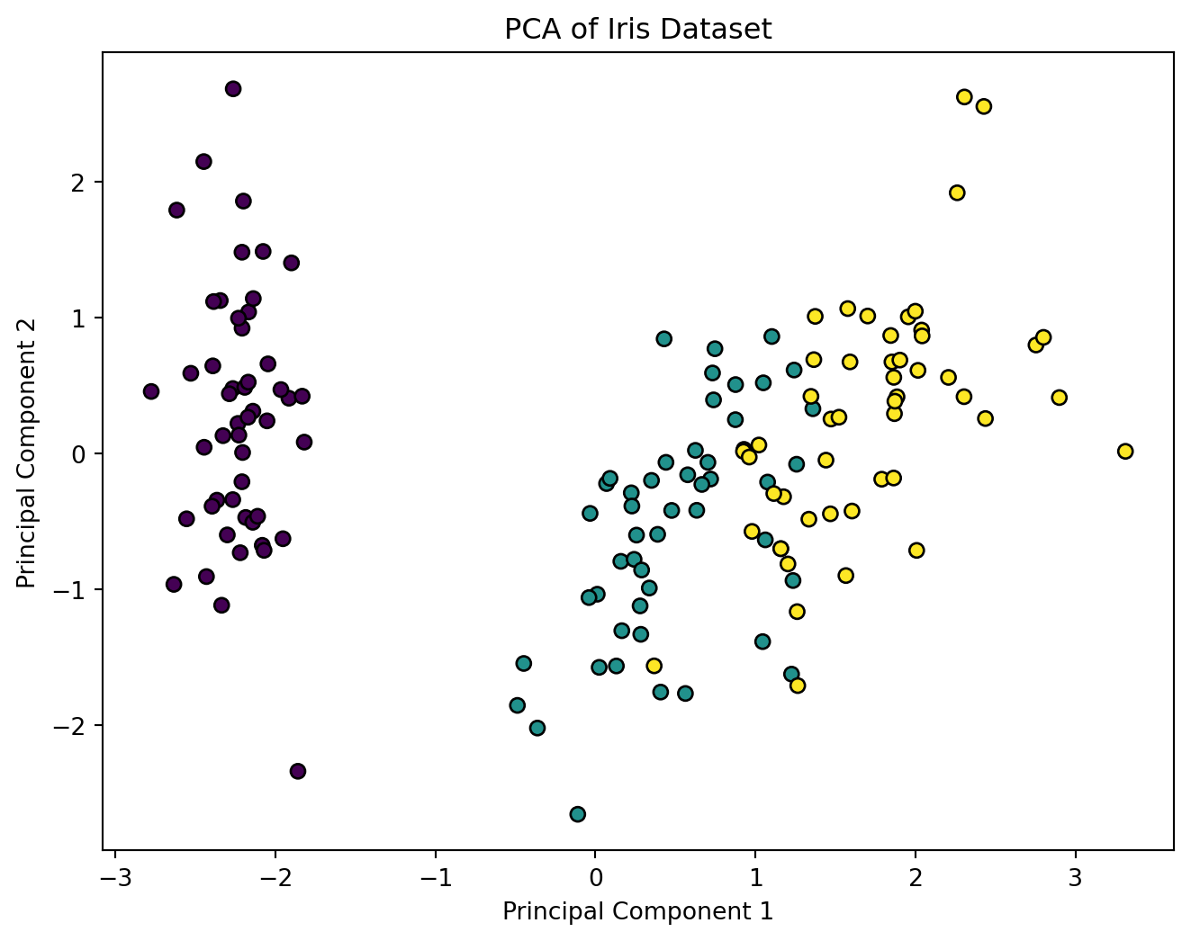
4.3 Python Code Example: Applying PCA in scikit-learn
Let’s see how the PCA process works in practice using Python’s scikit-learn library.