In this chapter, we extend PCA on weighted data by incorporating a metric matrix\(\mathbf{M}\) into the PCA process. The matrix \(\mathbf{M} \in \mathbb{R}^{p \times p}\) represents a metric applied to the feature space (also known as the individual space). This method allows us to take into account both the weights of observations and a metric that captures relationships between features.
The process involves two matrices:
\(\mathbf{D} \in \mathbb{R}^{n \times n}\), a diagonal matrix that assigns weights to each observation.
\(\mathbf{M} \in \mathbb{R}^{p \times p}\), a metric matrix on the feature space, typically representing the similarity or distance between features (e.g., Mahalanobis distance, covariance).
4.1 Motivation for Using a Metric \(\mathbf{M}\)
Introducing a metric \(\mathbf{M}\) on the feature space can be useful in the following scenarios:
Feature Correlations: Some features might be correlated, and a metric like the Mahalanobis distance can help account for those correlations.
Different Units: When features are measured in different units, a metric can standardize their importance in PCA.
Feature Relationships: In some cases, you might want to capture more complex relationships between features, which a custom metric can model.
4.2 Examples of \(\mathbf{D}\) and \(\mathbf{M}\)
4.2.1 Examples of Weight Matrix \(\mathbf{D}\)
The weight matrix \(\mathbf{D} \in \mathbb{R}^{n \times n}\) is a diagonal matrix, where:
Each diagonal element \(D_{ii}>0\) represents the weight assigned to the \(i\)-th observation;
And \(\sum_{i}D_{i,i}=1\).
Here are a few practical examples of how \(\mathbf{D}\) can be constructed.
4.2.1.1 Uniform Weighting
In the case where all observations are considered equally important, \(\mathbf{D}\) would be the identity matrix \(\dfrac{1}{n}\mathbf{I}\):
If certain observations are more precise or reliable than others, you might assign weights inversely proportional to the variance of each observation. For example, if the variance of observation \(i\) is \(\sigma_i^2\), then the weight for observation \(i\) could be \(D_{ii} \propto \frac{1}{\sigma_i^2}\):
This approach gives more weight to observations with lower variance (higher precision) and less weight to observations with higher variance (lower precision).
4.2.2 Examples of Metric Matrix \(\mathbf{M}\)
The metric matrix \(\mathbf{M} \in \mathbb{R}^{p \times p}\) represents a metric on the feature space (also known as the individual space). \(\mathbf{M}\) can account for feature correlations, scaling differences, or even custom-defined relationships between features. Here are a few common examples:
4.2.2.1 Identity Matrix (Euclidean Distance)
If you want to use the standard Euclidean distance in the feature space, the metric matrix \(\mathbf{M}\) is simply the identity matrix \(\mathbf{I}_p\):
In this case, all features are treated equally, and there is no special scaling or correlation between them.
4.2.2.2 Feature Scaling (Diagonal Matrix)
If the features have different units or ranges, you can use a diagonal matrix for \(\mathbf{M}\) where each diagonal element represents the inverse variance (or standard deviation) of the corresponding feature. This would apply feature scaling in the PCA process:
\[
M_{jj} = \frac{1}{\sigma_j^2}
\]
where \(\sigma_j^2\) is the variance of the \(j\)-th feature. For example, if there are three features with variances \(\sigma_1^2 = 2\), \(\sigma_2^2 = 5\), and \(\sigma_3^2 = 1\), the metric matrix would be:
The Mahalanobis distance takes into account the correlations between features and is commonly used when features are highly correlated. The metric matrix \(\mathbf{M}\) in this case is the inverse of the covariance matrix\(\mathbf{\Sigma}\) of the features:
\[
\mathbf{M} = \mathbf{\Sigma}^{-1}
\]
For example, if the covariance matrix \(\mathbf{\Sigma}\) is:
then the metric matrix \(\mathbf{M} = \mathbf{\Sigma}^{-1}\) is the inverse of this matrix, which can be computed using numerical methods.
The Mahalanobis distance is particularly useful in cases where features are correlated because it adjusts the PCA process to account for these correlations.
4.2.2.4 Custom Metric for Feature Importance
If you have domain knowledge indicating that some features are more important than others, you can create a custom metric matrix where larger weights are assigned to more important features. For example, if you want feature 2 to contribute twice as much as feature 1 and feature 3 to contribute half as much as feature 1, the matrix might look like:
This ensures that feature 2 has a larger impact on the PCA results, while feature 3 has a smaller impact.
4.2.3 Combined Example of \(\mathbf{D}\) and \(\mathbf{M}\)
Let’s put everything together. Suppose you are performing PCA on a dataset with 4 observations and 3 features. The diagonal weight matrix \(\mathbf{D}\) might represent inverse variance weights for the observations, and the metric matrix \(\mathbf{M}\) could represent a feature correlation structure.
Weight the observations using \(\mathbf{D}\), giving more importance to certain observations.
Account for feature correlations using the metric \(\mathbf{M}\).
4.3 Step-by-Step Procedure for PCA with \(\mathbf{D}\) and \(\mathbf{M}\)
Let \(\mathbf{X} \in \mathbb{R}^{n \times p}\) be the data matrix with \(n\) observations (rows) and \(p\) features (columns). Let:
\(\mathbf{D} \in \mathbb{R}^{n \times n}\) be the diagonal weight matrix that assigns weights to observations.
\(\mathbf{M} \in \mathbb{R}^{p \times p}\) be the metric matrix that applies to the features.
The steps for performing PCA with both weighted data and a metric are as follows:
4.3.1 Step 1: Center the Data Using Weighted Means
The first step is to center the data matrix \(\mathbf{X}\) using the weighted mean for each feature. The weighted mean for each feature \(j\) is computed as:
4.3.2 Step 2: Apply the Metric Matrix \(\mathbf{M}\) to the Feature Space
Now, we incorporate the metric matrix \(\mathbf{M}\) into the PCA process. The metric matrix can be used to transform the feature space and account for correlations or differences in scale between features.
Incorporating \(\mathbf{M}\) transforms the data matrix \(\mathbf{X}_c\) as follows:
where \(\mathbf{M}^{1/2}\) is the square root of the metric matrix \(\mathbf{M}\), which ensures that the transformation is applied correctly. This transformation maps the original features into a new space that respects the metric \(\mathbf{M}\).
4.3.3 Step 3: Compute the Weighted Covariance Matrix with the Metric
Next, we compute the weighted covariance matrix\(S_w^2\) with the metric. The weighted covariance matrix is given by:
This covariance matrix takes into account both the observation weights (from \(\mathbf{D}\)) and the feature relationships (from \(\mathbf{M}\)).
4.3.4 Step 4: Perform Eigenvalue Decomposition on the Weighted Covariance Matrix
Next, we perform eigenvalue decomposition on the weighted covariance matrix \(S_w^2\). This step gives us the eigenvalues and eigenvectors of the weighted covariance matrix:
\[
S_w^2 \mathbf{v}_i = \lambda_i \mathbf{v}_i
\]
where:
\(\mathbf{v}_i\) is an eigenvector of \(S_w^2\) (also called a principal component).
\(\lambda_i\) is the corresponding eigenvalue, representing the amount of variance along the direction of \(\mathbf{v}_i\).
4.3.5 Step 5: Select Principal Components
Once we have the eigenvalues and eigenvectors, we can select the principal components based on the explained variance. The total weighted variance is the sum of the eigenvalues:
You can use the explained variance ratio to determine how many principal components to retain.
4.3.6 Step 6: Project Data onto Principal Components
Finally, after selecting the top \(k\) principal components, we project the transformed data \(\mathbf{X}_M\) onto these components to reduce the dimensionality. Let \(\mathbf{V}_k \in \mathbb{R}^{p \times k}\) be the matrix containing the top \(k\) eigenvectors. The reduced data matrix \(\mathbf{X}_{\text{proj}} \in \mathbb{R}^{n \times k}\) is obtained by projecting the centered and transformed data onto the selected components:
This produces a new dataset where each observation is represented by \(k\) principal components.
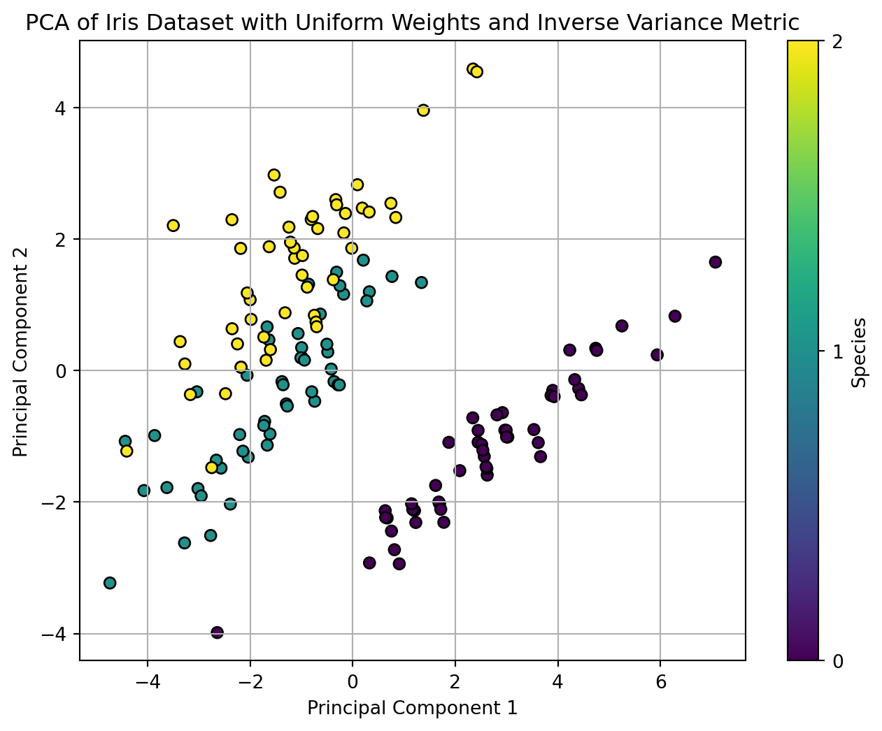
4.4 Python Code Example: PCA on Weighted Data with a Metric
Let’s look at an example of how to implement PCA on weighted data with a metric \(\mathbf{M}\) in Python.
import numpy as npimport matplotlib.pyplot as pltfrom sklearn.datasets import load_irisfrom sklearn.preprocessing import StandardScaler# Load Iris datasetdata = load_iris()X = data.datay = data.target# Number of observations (n) and number of features (p)n, p = X.shape# Step 1: Center datascaler = StandardScaler(with_mean =True)X_centered = scaler.fit_transform(X)# Step 2: Compute the diagonal metric matrix M with the inverses of variances on the diagonalvariances = np.var(X, axis=0, ddof=1) # Variances of the featuresM = np.diag(1/ variances) # Inverse of the variances# Step 3: Create uniform weights (D matrix) - here all weights are 1, so D is identity matrixD = np.eye(n)/n # Uniform weights: Identity matrix# Step 4: Apply the metric matrix to transform the dataX_transformed = X_centered @ np.sqrt(M) # Apply the square root of M to transform feature space# Step 5: Compute the weighted covariance matrixcov_matrix_weighted = X_transformed.T @ D @ X_transformed# Step 6: Perform eigenvalue decomposition on the weighted covariance matrixeigenvalues, eigenvectors = np.linalg.eigh(cov_matrix_weighted)# Step 7: Sort the eigenvalues and eigenvectors in descending ordersorted_idx = np.argsort(eigenvalues)[::-1]eigenvalues = eigenvalues[sorted_idx]eigenvectors = eigenvectors[:, sorted_idx]# Step 8: Project the data onto the top 2 principal componentsX_projected = X_transformed @ eigenvectors[:, :2]# Step 9: Plot the PCA resultplt.figure(figsize=(8,6))scatter = plt.scatter(X_projected[:, 0], X_projected[:, 1], c=y, cmap='viridis', edgecolor='k')plt.xlabel('Principal Component 1')plt.ylabel('Principal Component 2')plt.title('PCA of Iris Dataset with Uniform Weights and Inverse Variance Metric')plt.colorbar(scatter, ticks=[0, 1, 2], label='Species')plt.grid(True)plt.show()# Display the explained variance ratiosexplained_variances = eigenvalues / np.sum(eigenvalues)print(f"Explained variance ratios: {explained_variances[:2]}")