1  Introduction to PCA

1.1 Motivation and Intuition

Principal Component Analysis (PCA) is one of the most widely used techniques for dimensionality reduction. When dealing with large datasets with many features (high-dimensional data), visualizing and processing the data can become difficult. PCA helps by reducing the number of dimensions while retaining the most important information about the data, such as its variance.

Some common applications of PCA include:

• Data compression: Reducing the size of a dataset without significant loss of information.
• Noise reduction: Eliminating less informative features (dimensions) that may be noisy.
• Data visualization: Enabling easier visualization of data in 2D or 3D.
• Feature extraction: Selecting a subset of important features from a large set.

Let’s first ask, why do we need PCA? The curse of dimensionality refers to problems that arise when analyzing data in high-dimensional spaces, where the volume of the space grows exponentially with the number of dimensions. PCA is a powerful tool to combat these problems by reducing the dimensionality and summarizing the data.

1.1.1 The Curse of Dimensionality

As the number of dimensions increases:

• The data points become more spread out, making it hard to find patterns.
• Machine learning models may become more prone to overfitting.
• Visualization becomes impossible beyond 3 dimensions.

PCA offers a way to compress data, reduce noise, and identify the directions (or axes) where the data varies the most.

1.2 Learning Goals

In this chapter, you will learn:

• The intuition behind PCA and why it is important.
• How PCA reduces dimensionality while preserving important information in the data.
• The types of problems and datasets where PCA is useful.

PCA helps in compressing high-dimensional data while maintaining its most important characteristics.

Note

PCA can be viewed as a way to transform data into a new coordinate system where the first few coordinates (principal components) explain most of the variance in the data.

1.3 Key Terminology

Before diving into PCA, let’s briefly define some key terms that will be frequently used:

Definition 1.1 (Variance) Variance is a measure of how much the data points spread out from the mean in a given dataset. In PCA, we are particularly interested in finding directions (principal components) where the variance is maximized.

Definition 1.2 (Covariance) Covariance indicates how two variables change together. If variables increase together, the covariance is positive; if one decreases while the other increases, it is negative. PCA is based on the covariance matrix, which captures the covariance between different features in the data.

Definition 1.3 (Eigenvalues and Eigenvectors) Eigenvalues and eigenvectors play a central role in PCA. Eigenvectors represent the directions of maximum variance (principal components), and eigenvalues represent the amount of variance along those directions.

1.4 Applications of PCA

PCA is widely used in various fields. Some popular applications include:

• Image compression and recognition: PCA is often used to reduce the dimensionality of image datasets, such as in face recognition.
• Data visualization: When dealing with high-dimensional datasets (e.g., gene expression data), PCA can help in visualizing the data by projecting it onto a lower-dimensional space.
• Finance and economics: PCA is used to identify the underlying factors that explain correlations between various financial instruments.
• Bioinformatics: PCA is used to analyze high-dimensional biological data, like gene expression profiles or protein activity levels.

1.4.1 Example: Visualizing PCA

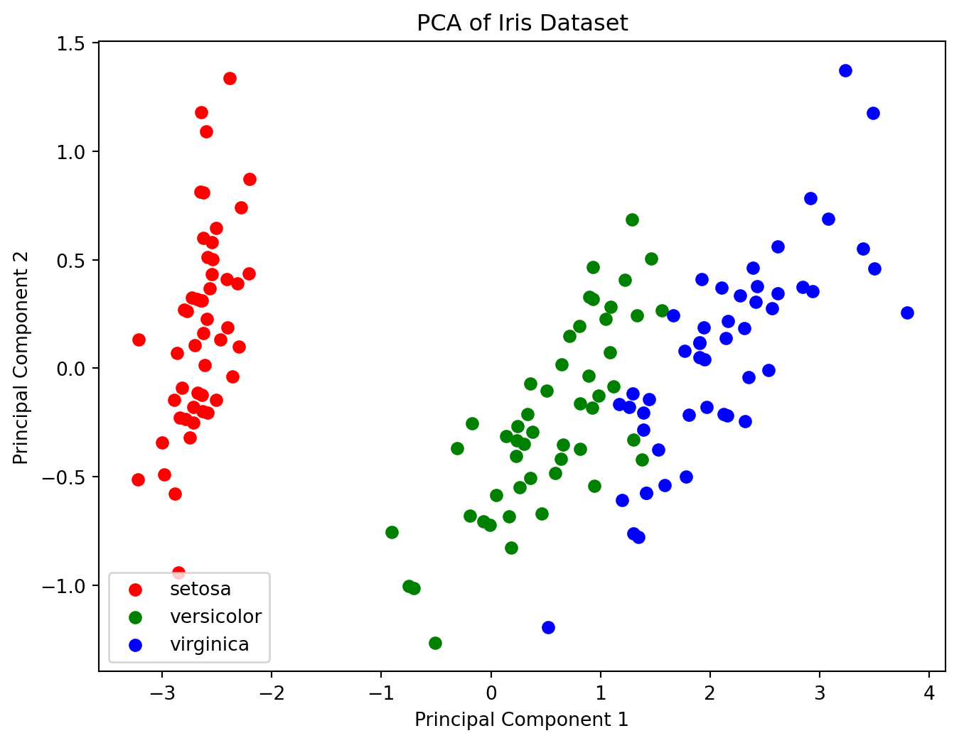
In high-dimensional spaces, it is often hard to understand the structure of the data. PCA can be used to project the data into 2D or 3D for visualization. For instance, when working with the famous Iris dataset, which contains 4 features, PCA can help reduce it to 2 principal components for easy visualization.

Here’s an example of PCA applied to the Iris dataset, visualizing the data in 2D:

import matplotlib.pyplot as plt
from sklearn.decomposition import PCA
from sklearn.datasets import load_iris
import pandas as pd

# Load dataset
iris = load_iris()
X = iris.data
y = iris.target

# Apply PCA
pca = PCA(n_components=2)
X_pca = pca.fit_transform(X)

# Convert to DataFrame for easy plotting
df_pca = pd.DataFrame(X_pca, columns=['PC1', 'PC2'])
df_pca['species'] = y

# Plotting
plt.figure(figsize=(8,6))
colors = ['r', 'g', 'b']
for i in range(3):
    plt.scatter(df_pca[df_pca['species'] == i]['PC1'], 
                df_pca[df_pca['species'] == i]['PC2'], 
                label=iris.target_names[i], 
                color=colors[i])
    
plt.title('PCA of Iris Dataset')
plt.xlabel('Principal Component 1')
plt.ylabel('Principal Component 2')
plt.legend()
plt.show()