Weights \(D\in\mathbb{R}^{n\times n}\) (diagonal matrix with weights \(d_i\))
The key transformation is:
\[Y = D^{1/2}XM^{1/2}\]
Then the SVD of \(Y\) gives us all PCA elements:
\[Y = U\Sigma V^T\]
Let’s implement this transformation:
Code
import numpy as npfrom scipy import linalgdef transform_for_svd(X, M, D):""" Transform data matrix for SVD computation Parameters: ----------- X : array-like, shape (n_samples, n_features) Data matrix M : array-like, shape (n_features, n_features) Metric matrix D : array-like, shape (n_samples, n_samples) Weight matrix (diagonal) Returns: -------- Y : array-like Transformed matrix for SVD """# Compute matrix square roots M_sqrt = linalg.sqrtm(M) D_sqrt = np.sqrt(D)# Transform X Y = np.diag(D_sqrt) @ X @ M_sqrtreturn Y# Example usagen, p =100, 5X = np.random.randn(n, p)M = np.eye(p) # Identity metricD = np.full(n, 1/n) # Uniform weightsY = transform_for_svd(X, M, D)
2.2 Recovering PCA Elements
From the SVD of \(Y\), we can recover all PCA elements:
Principal components: \(F = D^{-1/2}U\Sigma\)
Principal axes: \(A = M^{-1/2}V\)
Eigenvalues: \(\lambda_i = \sigma_i^2\)
Code
def compute_pca_from_svd(X, M, D):""" Compute PCA elements using SVD """# Transform data Y = transform_for_svd(X, M, D)# Compute SVD U, s, Vt = np.linalg.svd(Y, full_matrices=False)# Recover PCA elements M_sqrt = linalg.sqrtm(M) M_inv_sqrt = linalg.inv(M_sqrt) D_sqrt = np.sqrt(D)# Principal components F = np.diag(1/D_sqrt) @ U @ np.diag(s)# Principal axes A = M_inv_sqrt @ Vt.T# Eigenvalues eigenvals = s**2return F, A, eigenvals# Example with standardized datadef standardize(X):"""Standardize data matrix""" mean = X.mean(axis=0) std = X.std(axis=0)return (X - mean) / stdX_std = standardize(X)F, A, eigenvals = compute_pca_from_svd(X_std, M, D)
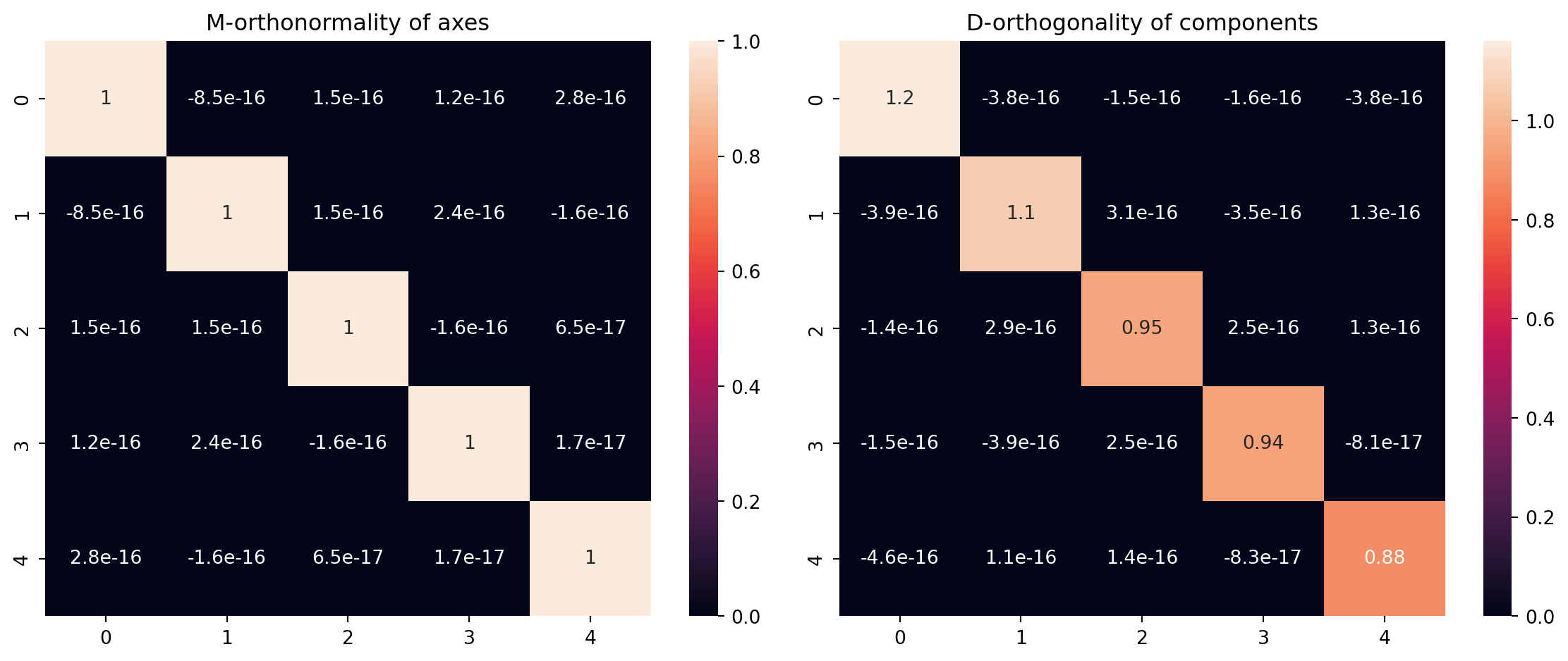
2.3 Properties and Verification
Let’s verify the key properties:
M-orthonormality of axes
D-orthogonality of components
Variance decomposition
Code
def verify_pca_properties(F, A, M, D):"""Verify PCA properties"""# M-orthonormality of axes axes_orthonormality = A.T @ M @ A# D-orthogonality of components components_orthogonality = F.T @ np.diag(D) @ Freturn axes_orthonormality, components_orthogonality# Verify propertiesaxes_ortho, comp_ortho = verify_pca_properties(F, A, M, D)import matplotlib.pyplot as pltimport seaborn as snsfig, (ax1, ax2) = plt.subplots(1, 2, figsize=(12, 5))sns.heatmap(axes_ortho, annot=True, ax=ax1)ax1.set_title('M-orthonormality of axes')sns.heatmap(comp_ortho, annot=True, ax=ax2)ax2.set_title('D-orthogonality of components')plt.tight_layout()plt.show()
2.4 Special Cases
2.4.1 Standard PCA
When \(M = I_p\) and \(D = \frac{1}{n}I_n\):
Code
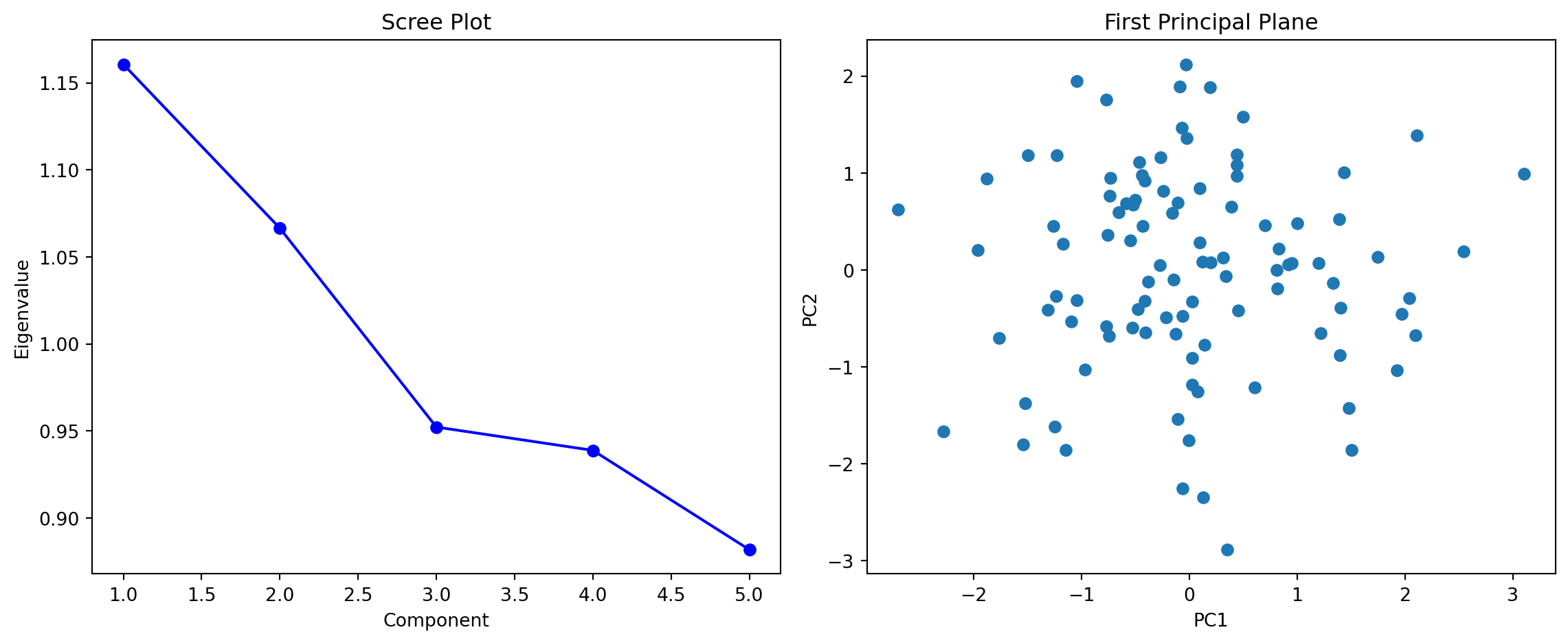
def standard_pca(X):"""Standard PCA with identity metric and uniform weights""" n = X.shape[0] M = np.eye(X.shape[1]) D = np.full(n, 1/n)return compute_pca_from_svd(X, M, D)# Compare with standard PCA implementationfrom sklearn.decomposition import PCApca_sklearn = PCA()pca_sklearn.fit(X_std)print("Eigenvalues from our implementation:", eigenvals)print("Eigenvalues from sklearn:", pca_sklearn.explained_variance_)
Eigenvalues from our implementation: [1.16057225 1.06647412 0.95225262 0.93887377 0.88182725]
Eigenvalues from sklearn: [1.1722952  1.07724658 0.96187133 0.94835734 0.89073459]
2.4.2 Normalized PCA
When \(M = \text{diag}(1/s_j^2)\) where \(s_j\) are variable standard deviations:
Code
def normalized_pca(X):"""PCA with variables normalized to unit variance""" std = X.std(axis=0) M = np.diag(1/std**2) n = X.shape[0] D = np.full(n, 1/n)return compute_pca_from_svd(X, M, D)