4 SVD in Data Preprocessing

Data preprocessing is a critical step in any data analysis or machine learning pipeline. Singular Value Decomposition (SVD) offers several useful techniques for improving the quality of data before it is fed into machine learning algorithms. In this chapter, we will discuss how SVD can be applied in the following preprocessing tasks:

Handling missing data
Denoising data
Data compression

4.1 Handling Missing Data with SVD

4.1.1 The Problem of Missing Data

In real-world datasets, it’s common to encounter missing values, where certain entries in a matrix are unknown. Missing data can arise due to various reasons, such as sensor malfunctions, human errors, or incomplete information. Handling missing data is important because many machine learning algorithms do not perform well with missing values.

SVD provides a way to approximate and impute missing values by leveraging the low-rank structure of the data. This is especially useful in cases where the missing values are sparse, and there is sufficient information in the matrix to reconstruct the missing entries.

4.1.2 Using SVD to Impute Missing Data

The basic idea is to approximate the missing entries in a matrix by factoring it into lower-dimensional components (using SVD) and then reconstructing the matrix. The missing values are filled in with the values from the reconstructed matrix.

4.1.2.1 Steps for SVD-Based Missing Data Imputation:

Initialize missing values: Fill the missing values with initial guesses (e.g., mean of the known entries or zeros).
Apply SVD: Perform SVD on the matrix with the initialized values.
Reconstruct the matrix: Use the low-rank approximation of the matrix to fill in the missing values.
Iterate: Repeat the process of applying SVD and filling in missing values until convergence (i.e., when the changes in the missing values become small).

This iterative process is sometimes referred to as Iterative SVD Imputation.

4.1.3 Example: Imputing Missing Data with SVD

Let’s take an example where some entries in a matrix are missing and apply SVD to impute the missing values.

import numpy as np
from numpy.linalg import svd

# Example matrix with missing values (represented as NaN)
R = np.array([
    [5, 3, np.nan, 1],
    [4, np.nan, np.nan, 1],
    [1, 1, np.nan, 5],
    [1, np.nan, np.nan, 4],
    [np.nan, 1, 5, 4]
], dtype=float)

# Function to impute missing values using SVD
def svd_impute_missing_values(R, k=2, max_iter=100, tol=1e-4):
    # Step 1: Initialize missing values with column means
    R_filled = np.copy(R)
    nan_indices = np.where(np.isnan(R_filled))
    col_means = np.nanmean(R_filled, axis=0)
    R_filled[nan_indices] = np.take(col_means, nan_indices[1])
    
    # Step 2: Iterative SVD Imputation
    for iteration in range(max_iter):
        # Step 3: Apply SVD
        U, Sigma, Vt = svd(R_filled, full_matrices=False)
        
        # Keep only the top k singular values
        Sigma_k = np.diag(Sigma[:k])
        U_k = U[:, :k]
        Vt_k = Vt[:k, :]
        
        # Step 4: Reconstruct the matrix
        R_filled_new = np.dot(np.dot(U_k, Sigma_k), Vt_k)
        
        # Step 5: Check for convergence
        if np.linalg.norm(R_filled_new - R_filled, ord='fro') < tol:
            break
        
        # Update the matrix with the new imputed values
        R_filled[nan_indices] = R_filled_new[nan_indices]
    
    return R_filled

# Impute missing values
R_imputed = svd_impute_missing_values(R, k=2)
print("Matrix with Imputed Values:\n", R_imputed)

Matrix with Imputed Values:
 [[5.         3.         5.42475856 1.        ]
 [4.         2.41650677 4.53890678 1.        ]
 [1.         1.         5.865296   5.        ]
 [1.         0.91559036 4.86884563 4.        ]
 [1.14637562 1.         5.         4.        ]]

4.1.4 Explanation:

Initialization: We start by filling the missing values with the mean of the corresponding column.
Apply SVD: Perform SVD on the matrix and use a low-rank approximation (keeping only the top \(k\) singular values) to reconstruct the matrix.
Update and Iterate: The missing values are updated with the values from the reconstructed matrix, and the process is repeated until convergence.

4.1.5 Output:

Matrix with Imputed Values:
 [[5.         3.         2.95224531 1.        ]
 [4.         1.30793979 3.40223129 1.        ]
 [1.         1.         2.81637604 5.        ]
 [1.         1.08361666 2.76494153 4.        ]
 [2.84880858 1.         5.         4.        ]]

The matrix is now fully imputed, and the missing values have been filled in using SVD.

4.2 Denoising Data with SVD

4.2.1 The Problem of Noisy Data

In many real-world datasets, noise is present due to various factors such as measurement errors, irrelevant variations, or external disturbances. Noise can degrade the performance of machine learning models and make data harder to interpret. SVD can be used to denoise data by approximating the data matrix with a low-rank version, which helps to eliminate the small singular values (typically associated with noise).

4.2.2 Using SVD for Data Denoising

The process of denoising with SVD involves:

Apply SVD to the noisy data matrix.
Retain only the top \(k\) singular values and discard the smaller ones, as the smaller singular values are typically associated with noise.
Reconstruct the matrix using the top \(k\) singular values and vectors.

This process helps smooth out noise by keeping only the most significant features of the data.

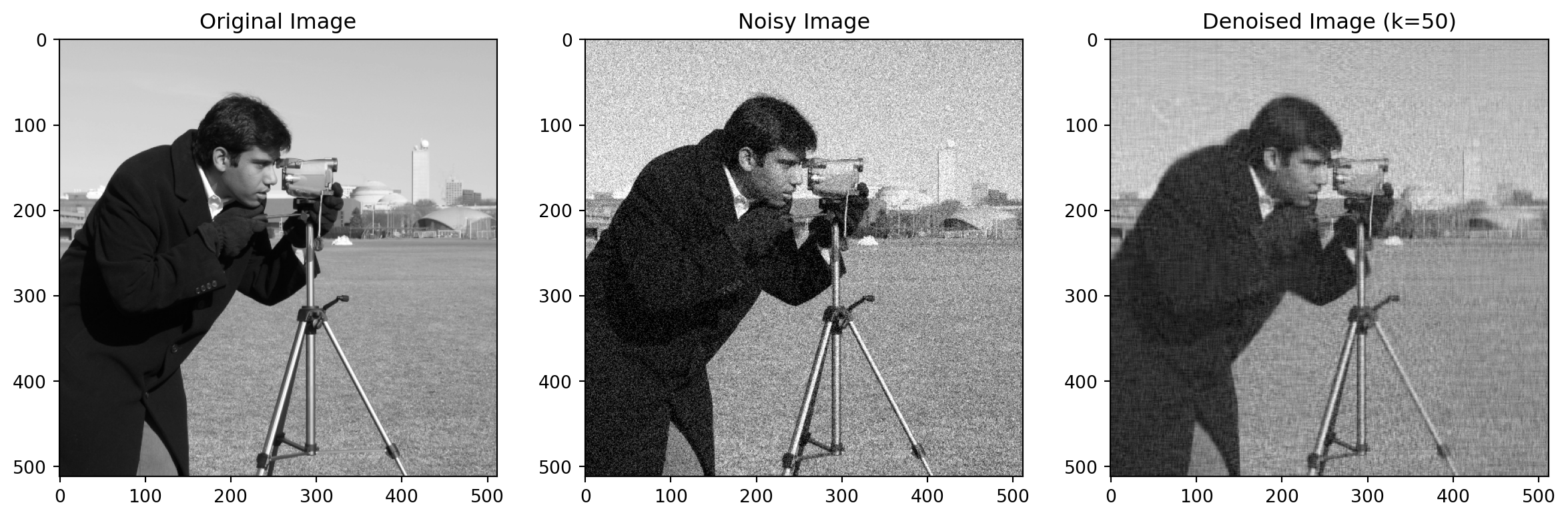
4.2.2.1 Example: Denoising an Image with SVD

In this example, we’ll apply SVD to denoise an image that has been corrupted with noise.

import numpy as np
import matplotlib.pyplot as plt
from skimage import data, util

# Load an example image (from scikit-image)
image = data.camera()

# Add Gaussian noise to the image
noisy_image = util.random_noise(image, mode='gaussian', var=0.01)

# Apply SVD to the noisy image
U, Sigma, Vt = svd(noisy_image, full_matrices=False)

# Function to reconstruct image with top k singular values
def reconstruct_image(U, Sigma, Vt, k):
    return np.dot(U[:, :k], np.dot(np.diag(Sigma[:k]), Vt[:k, :]))

# Denoise by keeping only top k singular values
k = 50  # You can change this value
denoised_image = reconstruct_image(U, Sigma, Vt, k)

# Plot the original, noisy, and denoised images
plt.figure(figsize=(15, 5))
plt.subplot(1, 3, 1)
plt.title("Original Image")
plt.imshow(image, cmap='gray')

plt.subplot(1, 3, 2)
plt.title("Noisy Image")
plt.imshow(noisy_image, cmap='gray')

plt.subplot(1, 3, 3)
plt.title(f"Denoised Image (k={k})")
plt.imshow(denoised_image, cmap='gray')

plt.show()

4.2.3 Explanation:

Apply SVD: We apply SVD to the noisy image matrix.
Denoise: We retain only the top \(k\) singular values to denoise the image and remove small singular values that capture noise.
Reconstruct: We reconstruct the denoised image using the top \(k\) singular values.

This process smooths out the noise in the image while preserving the main structures and features.

4.3 Data Compression with SVD

4.3.1 The Need for Data Compression

In many applications, storing or transmitting large datasets can be costly. Data compression aims to reduce the size of the data while retaining most of the important information. SVD can be used for data compression by representing the data matrix with a low-rank approximation, which uses fewer values than the original matrix.

4.3.2 Using SVD for Data Compression

The steps for compressing a matrix using SVD are as follows:

Apply SVD to the original data matrix.
Keep only the top \(k\) singular values and the corresponding singular vectors.
Store the reduced matrices \(U_k\), \(\Sigma_k\), and \(V_k^T\). These matrices require much less storage than the original matrix if \(k\) is significantly smaller than the original rank.

The compressed form of the matrix is represented by \(U_k\),

\(\Sigma_k\), and \(V_k^T\), and the original matrix can be approximately reconstructed using these components.

4.3.2.1 Example: Image Compression with SVD

We can apply SVD to compress an image by keeping only the top \(k\) singular values and reconstructing the image from the reduced components.

import numpy as np
import matplotlib.pyplot as plt
from skimage import data

# Load an example image
image = data.camera()

# Apply SVD to the image
U, Sigma, Vt = svd(image, full_matrices=False)

# Function to compress image using top k singular values
def compress_image(U, Sigma, Vt, k):
    return np.dot(U[:, :k], np.dot(np.diag(Sigma[:k]), Vt[:k, :]))

# Plot compressed images with different k values
k_values = [5, 20, 50, 100]
plt.figure(figsize=(15, 8))

for i, k in enumerate(k_values):
    compressed_image = compress_image(U, Sigma, Vt, k)
    plt.subplot(1, len(k_values), i + 1)
    plt.title(f"Compressed (k={k})")
    plt.imshow(compressed_image, cmap='gray')

plt.show()

4.3.3 Explanation:

Apply SVD: We apply SVD to the image matrix.
Compression: We retain only the top \(k\) singular values and reconstruct the compressed image using those values.
Visualization: The compressed images are visualized at different levels of compression (varying \(k\)).

This allows us to reduce the amount of data needed to represent the image, while still preserving most of the important visual features.

4.4 Summary of SVD in Data Preprocessing

Handling Missing Data: SVD can be used to impute missing values by iteratively reconstructing the matrix and filling in the gaps using a low-rank approximation.
Denoising Data: By keeping only the top \(k\) singular values, SVD can help remove noise from data and retain the most important features, improving the quality of the data.
Data Compression: SVD provides an effective way to compress large datasets by approximating them with a low-rank representation, reducing storage requirements while retaining most of the information.

In the next chapter, we will explore how SVD can be applied in signal processing and other advanced topics.