Bivariate analysis

Bivariate statistics delve deeper into data analysis by examining the relationship between two variables. They help us understand how changes in one variable might be associated with changes in another. Essentially, it goes beyond looking at each variable in isolation and instead focuses on exploring potential connections between them.

Here’s a breakdown of key points about bivariate statistics:

• Focus: Analyzes the relationship between two variables.
• Objective: To understand how changes in one variable might be linked to changes in another.
• Outcomes: Provides insights into the strength, direction, and type of the relationship between the two variables.
• Applications: Used in various fields like research, marketing, finance, and social sciences to understand how variables interact.

Two Numeric Variables

• Data: \((x_i, y_i)\in\mathbb{R}^2\), where \(i = 1, 2, \cdots, n\)

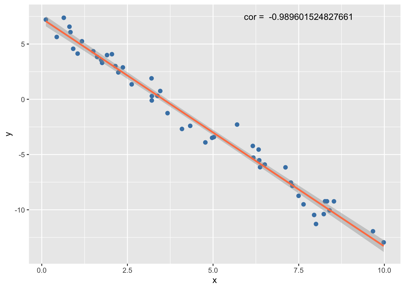
Pearson Correlation Coefficient

• Measures the strength and direction of the linear relationship between \(X\) and \(y\).

\[r_{x,y} = \dfrac{\sum_{i=1}^{n} (x_i - \bar{x}) (y_i - \bar{y})} {\sqrt{\sum_{i=1}^{n} (x_i - \bar{x})^2 \sum_{i=1}^{n} (y_i - \bar{y})^2}}\] where

• \(\bar{x}=\dfrac{1}{n}\sum_{i=1}^nx_i\) is the mean of \(X\)
• \(\bar{y}=\dfrac{1}{n}\sum_{i=1}^ny_i\) is the mean of \(Y\).

Interpretation

• \(r_{x,y}\in\left[-1,1\right]\);

• \(r_{x, y}\in\left\{-1,1\right\}\): perfect correlation;

• \(r_{x,y}\) is closer to \(1\) as the linear relationship between \(X\) and \(Y\) is stronger;

• \(r_{x,y}\approx 0\): No linear relationship.

Covariance

• Measures the direction and magnitude of the linear dependence between \(X\) and \(Y\), regardless of the units of measurement.

\[ \begin{aligned} S_{x,y} &= \dfrac{1}{n}\sum_{i=1}^{n} (x_i - \bar{x}) (y_i - \bar{y})\\ &=\dfrac{1}{n}\sum_{i=1}^nx_iy_i-\bar{x}\bar{y} \end{aligned} \]

Interpretation

• A positive covariance suggests both variables tend to move in the same direction (increasing or decreasing together).
• A negative covariance suggests they tend to move in opposite directions.
• A covariance of zero indicates no linear dependence.

Remarks

• \(r_{x,y}=\dfrac{S_{x,y}}{S_xS_y}\) where \(S_x\) and \(S_y\) are the standard deviations or \(X\) and \(Y\).

Scatter Plot

• A visual representation of the relationship between \(X\) and \(Y\), where each data point \((x_i, y_i)\) is plotted.
• The scatter plot helps identify potential patterns like linear trends, clusters, or non-linear relationships.

Example 1 (Linear relationship)  

Additional Considerations:

• Non-linear relationships: While correlation and covariance focus on linear relationships, other techniques may be needed to explore non-linear relationships.
• Outliers: Outliers can significantly influence bivariate statistics. It’s crucial to identify and handle outliers appropriately before interpreting the results.

Analysis of Two Categorical Variables

When analyzing relationships between two categorical variables \(X\) and \(Y\), we denote the levels of \(X\) by \(a_k\), where \(k = 1, \ldots, K\), and the levels of \(Y\) by \(b_l\), where \(l = 1, \ldots, L\). This notation allows us to flexibly describe the categories of each variable.

Contingency Table

A contingency table represents the frequency of observations for each combination of the levels of \(X\) and \(Y\):

	\(b_1\ \)	\(b_2\ \)	\(\cdots\ \)	\(b_L\ \)	Total
\(a_1\)	\(n_{1,1}\)	\(n_{1,2}\)	\(\ldots\)	\(n_{1,L}\)	\(n_{1,+}\)
\(a_2\)	\(n_{2,1}\)	\(n_{2,2}\)	\(\ldots\)	\(n_{2,L}\)	\(n_{2,+}\)
\(\vdots\)	\(\vdots\)	\(\vdots\)	\(\ddots\)	\(\vdots\)	\(\vdots\)
\(a_K\)	\(n_{K,1}\)	\(n_{K,2}\)	\(\ldots\)	\(n_{K,L}\)	\(n_{K,+}\)
Total	\(n_{+,1}\)	\(n_{+,2}\)	\(\ldots\)	\(n_{+,L}\)	\(N\)

Where: - \(n_{kl}\) represents the observed frequency for level \(a_k\) of \(X\) and level \(b_l\) of \(Y\). - \(n_{k\cdot}\) is the total frequency for level \(k\) of \(X\) across all levels of \(Y\). - \(n_{\cdot l}\) is the total frequency for level \(l\) of \(Y\) across all levels of \(X\). - \(N\) is the grand total of all observations.

Chi-square statistic

The Chi-square statistic (\(\chi^2\)) is calculated as:

\[ \begin{aligned} \mathbb{X}^2 &= \sum_{k=1}^{K} \sum_{l=1}^{L} \dfrac{(n_{k,l} - E_{k,l})^2}{E_{k,l}} \end{aligned} \]

Where \(E_{k,l}\) is the expected frequency for each cell, calculated under the assumption of independence between \(X\) and \(Y\):

\[ E_{k,l} = \dfrac{n_{k\cdot} \times n_{\cdot l}}{n} \]

Cramer’s V

Cramer’s V is a measure of association strength between \(X\) and \(Y\), calculated as:

\[ V = \sqrt{\dfrac{\mathbb{X}^2 }{n\min(K-1, L-1)}} \]

This provides a value in \(]0, 1[\): The relationship is stronger as the \(V\) is close to \(1\).

Interpretation

For interpreting Cramér’s V, a measure of association between two categorical variables, the following thresholds can serve as a general guide:

• Very weak association: \(0.0 < V \leq 0.1\)
  • Negligible association between the variables, with minimal practical significance.
• Weak association: \(0.1 < V \leq 0.2\)
  • A slight association exists, but it’s weak and might not always be of practical importance.
• Moderate association: \(0.2 < V \leq 0.4\)
  • Indicates a moderate level of association, suggesting some relationship that could be of interest, depending on the context.
• Relatively strong association: \(0.4 < V \leq 0.6\)
  • A relatively strong association that suggests a substantial link, indicating that changes in one variable are related to changes in the other to a significant degree.
• Strong association: \(0.6 < V \leq 0.8\)
  • A strong association, suggesting a high likelihood that knowing the value of one variable gives considerable information about the value of the other.
• Very strong association: \(0.8 < V \leq 1.0\)
  • A very strong association, nearing a perfect relationship where the value of one variable almost perfectly predicts the value of the other.

Chi-square test of independance

• Hypothesis

• \(\left(\mathcal{H}_0\right)\): \(X\) and \(Y\) are independant
• \(\left(\mathcal{H}_1\right)\): \(X\) and \(Y\) are not independant

• Test statistic: \[ \mathbb{X}^2\overset{\left(\mathcal{H}_0\right)}{\sim}\chi_{(K-1)(L-1)}^2 \]

• Critical region at level \(\alpha\): \(W=\left]q_{1-\alpha}\left(\chi_{(K-1)(L-1)}^2\right),+\infty\right[\)

• p-value: \(pValue=\mathbb{P}\left(\chi_{(K-1)(L-1)}^2>\mathbb{X}_{obs}^2\right)\)

• Reject \(\left(\mathcal{H}_0\right)\) if and only if \[ \begin{aligned} \mathbb{X}_{obs}^2 \in W &\equiv \mathbb{X}_{obs}^2>q_{1-\alpha}\left(\chi_{(K-1)(L-1)}^2\right)\\ &\equiv pValue <\alpha\\ \end{aligned} \]

One numeric and one categorical variables

The categorical variable create a partition of the quantitative data into \(K\) classes, each associated with one level. Let denote by:

• \(x_{i,k}\) as the observation of the numeric variable on individual \(i\) in class \(k\)th

• \(n_k\) the number of individual in class \(k\)th

• Then the overall sample size is \(n=\sum_{k=1}^Kn_k\)

Means

• Mean of \(X\) in the \(k\)th class: \[ \bar{x}_k=\dfrac{1}{n_k}\sum_{i=1}^{n_k}x_{i,k}. \]

• Overall mean \[ \bar{x}=\dfrac{1}{n}\sum_{k=1}^Kn_k\bar{x}_k. \]

Sum of squares

• Within sum of squares \[ WSS = \sum_{k=1}^K\left(x_{i, k}-\bar{x}_k\right)^2 \]

• Between sum of squares

\[ BSS = \sum_{k=1}^Kn_k\left(\bar{x}_k-\bar{x}\right)^2 \]

• Total sum of squares \[ \begin{aligned} TSS &=\sum_{k=1}^K\sum_{i=1}^{n_k}\left(x_{i,k}-\bar{x}\right)^2\\ &= WSS+BSS\\ \end{aligned} \]

Variances

• Within variance \[ WV=\dfrac{WSS}{n-K} \]
• Between variance \[ BV=\dfrac{BSS}{K-1} \]
• Total variance \[ TV = \dfrac{TSS}{n-1} \]

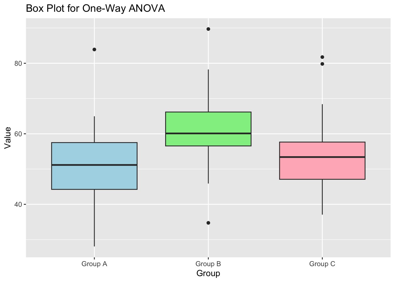
One way ANOVA

One-way ANOVA (Analysis of Variance) is a statistical method used to test if there are any statistically significant differences between the means of the \(K>2\) independent (unrelated) groups. This method is based on comparing the variance (variability) within groups against the variance between groups. If the between-group variance is significantly larger than the within-group variance, it suggests that at least one group mean is different from one another. The “one-way” aspect of ANOVA refers to analyzing the influence of a single independent variable (factor) on a continuous dependent variable. It’s a useful technique in research for determining the effect of different treatments, conditions, or classifications on a subject of interest.

Let denote by \(\mu_k=\mathbb{E}\left[X_{i,k}\right]\) the expectation of the quantitative variable in class \(k\).

Hypothesis

• \(\left(\mathcal{H}_0\right)\): \(\mu_1=\cdots=\mu_k=\cdots=\mu_K\)
• \(\left(\mathcal{H}_1\right)\): \(\exists k,l|\ \mu_k\neq\mu_l\)

Test statistic

\[ F=\dfrac{BV}{WB}\overset{\left(\mathcal{H}_0\right)}{\sim}\mathcal{F}_{K-1, n-K}. \]

P-value

\[ pValue=\mathbb{P}\left(\mathcal{F}_{K-1, n-K}>F_{obs}\right) \]

Decision

Reject \(\left(\mathcal{H}_0\right)\) if and only \(F_{obs}>q_{1-\alpha}\left(\mathcal{F}_{K-1, n-K}\right)\) or \(pValue<\alpha\).

Source	Dof	SS	Variance	F-Statistic	P-value
Between	\(K-1\)	\(BSS\)	\(BV=\dfrac{BSS}{K-1}\)	\(F=\dfrac{BV}{WV}\)	\(pValue\)
Within	\(n-K\)	\(WSS\)	\(WV=\dfrac{WSS}{n-K}\)	-	-
Total	\(n-K-1\)	\(TSS\)	-	-	-

• Dof: Degrees of freedom

• SS: Sum of squares

Example 2 (One way anova)  

             Df Sum Sq Mean Sq F value   Pr(>F)    
group         2   2685  1342.3   14.72 1.48e-06 ***
Residuals   147  13401    91.2                     
---
Signif. codes:  0 '***' 0.001 '**' 0.01 '*' 0.05 '.' 0.1 ' ' 1