4 Applications of SVD

Singular Value Decomposition (SVD) is a powerful matrix decomposition technique that has numerous applications in data analysis, machine learning, signal processing, and more. In this chapter, we will explore some of the most important applications of SVD in practical contexts.

4.1 Low-Rank Approximation

One of the key applications of SVD is low-rank approximation, which allows us to approximate a matrix \(A \in \mathbb{R}^{n \times p}\) by another matrix of lower rank \(k\). This is particularly useful for reducing the storage and computational complexity of large datasets.

4.1.1 Best Rank-\(k\) Approximation

Given the SVD of a matrix \(A = U \Sigma V^T\), the rank-\(k\) approximation of \(A\), denoted as \(A_k\), is obtained by truncating the SVD:

\[ A_k = U_k \Sigma_k V_k^T \]

where:

\(U_k\) consists of the first \(k\) columns of \(U\),
\(\Sigma_k\) is a diagonal matrix containing the largest \(k\) singular values,
\(V_k\) consists of the first \(k\) columns of \(V\).

This approximation minimizes the Frobenius norm:

\[ \| A - A_k \|_F \]

and is the best approximation of rank \(k\) in terms of capturing the maximum variance of the data.

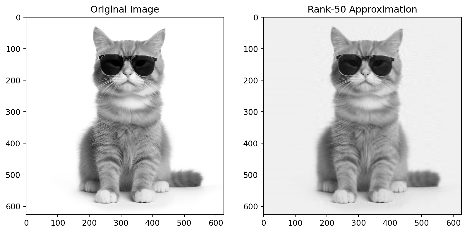
4.1.2 Example: Image Compression

Images can be represented as large matrices where each entry corresponds to the intensity of a pixel. Using SVD, we can create a low-rank approximation of an image that retains most of the visual features while reducing storage size.

import numpy as np
import matplotlib.pyplot as plt
from scipy.linalg import svd

# Load an example image
image = plt.imread('cat.png')

# Convert the image to grayscale (optional)
image_gray = np.mean(image, axis=2)

# Perform SVD
U, Sigma, Vt = svd(image_gray, full_matrices=False)

# Create a rank-k approximation (k=50)
k = 50
image_approx = np.dot(U[:, :k], np.dot(np.diag(Sigma[:k]), Vt[:k, :]))

# Display original and compressed images
plt.figure(figsize=(10,5))

plt.subplot(1, 2, 1)
plt.imshow(image_gray, cmap='gray')
plt.title("Original Image")

plt.subplot(1, 2, 2)
plt.imshow(image_approx, cmap='gray')
plt.title(f"Rank-{k} Approximation")

plt.show()

In this example:

The original image is represented by a matrix \(A\).
We compute its SVD, retain the largest 50 singular values, and reconstruct the image using the rank-50 approximation.
The result is a compressed version of the original image, with significantly fewer values.

Compression Ratio

The compression ratio is the ratio of the number of stored values in the approximated image \(A_q\) to the number of stored values in the original image \(A\):

\[ \text{Compression Ratio} = \dfrac{q (m + n + 1)}{m n} \]

Where: - \(q\) is the number of singular values retained, - \(m \times n\) is the size of the original matrix \(A\).

4.2 Principal Component Analysis (PCA)

Principal Component Analysis (PCA) is a widely-used dimensionality reduction technique that can be computed using the SVD. Given a centered data matrix \(X\), the PCA of \(X\) can be derived from the SVD:

\[ X = U \Sigma V^T \]

The right singular vectors (columns of \(V\)) are the principal components, and the singular values in \(\Sigma\) represent the amount of variance explained by each principal component.

4.2.1 PCA and Dimensionality Reduction

By keeping only the first few principal components, we can reduce the dimensionality of the dataset while preserving most of the variability. This is particularly useful for large datasets with many features, such as gene expression data or image data.

4.2.2 Example: PCA with SVD in Python

import numpy as np
from sklearn.decomposition import PCA

# Generate synthetic data
np.random.seed(0)
X = np.random.rand(100, 10)

# Perform PCA using SVD
U, Sigma, Vt = svd(X - np.mean(X, axis=0), full_matrices=False)
principal_components = Vt.T

# Display the first two principal components
print("First two principal components:", principal_components[:, :2])

First two principal components: [[-0.07325208 -0.46047999]
 [ 0.5616889   0.09677487]
 [-0.09734634 -0.07824592]
 [ 0.39215191 -0.38452405]
 [-0.14119616 -0.29517307]
 [ 0.17690769 -0.60626834]
 [ 0.33303421  0.18071889]
 [ 0.36140944  0.12428128]
 [ 0.43620395  0.16373674]
 [-0.18123228  0.3082342 ]]

In this example, we compute the principal components using the SVD of the data matrix \(X\).

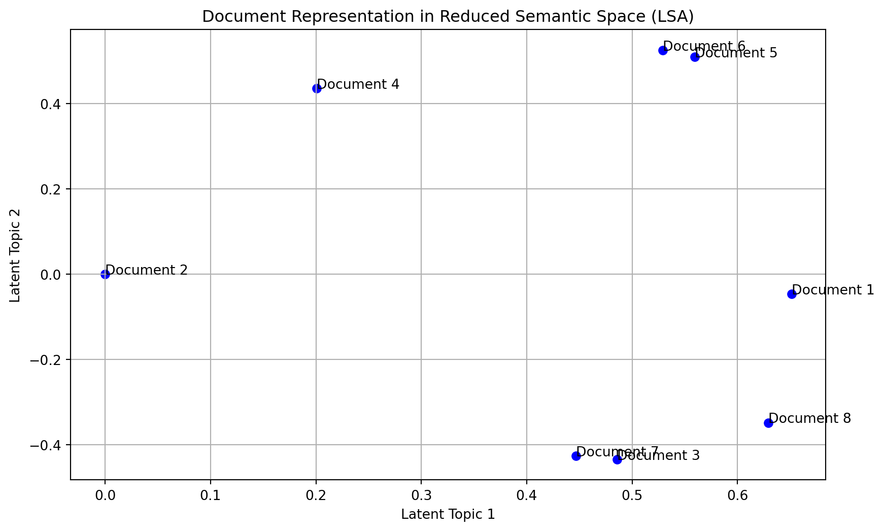
4.3 Latent Semantic Analysis (LSA)

Latent Semantic Analysis (LSA) is a technique used in natural language processing (NLP) to uncover relationships between terms and documents in a text corpus. It is based on the SVD of a term-document matrix \(A\), where rows represent terms and columns represent documents.

After performing the SVD of \(A\):

\[ A = U \Sigma V^T \]

The matrix \(U\) represents terms, \(V\) represents documents, and \(\Sigma\) captures important latent relationships between terms and documents.

4.3.1 Example: Latent Semantic Analysis

from sklearn.feature_extraction.text import CountVectorizer
from sklearn.decomposition import TruncatedSVD

# Example text data
documents = [
    "SVD is useful for dimensionality reduction",
    "PCA is a common application of SVD",
    "SVD can be used for text analysis",
    "LSA uncovers relationships in text"
]

# Convert the text data into a term-document matrix
vectorizer = CountVectorizer()
X = vectorizer.fit_transform(documents)

# Perform Latent Semantic Analysis (LSA) using SVD
lsa = TruncatedSVD(n_components=2)
X_lsa = lsa.fit_transform(X)

print("LSA representation:", X_lsa)

LSA representation: [[ 1.84075866 -0.67936622]
 [ 1.49588372 -1.35873244]
 [ 1.99950577  1.35873244]
 [ 0.41675728  1.35873244]]

import numpy as np
import matplotlib.pyplot as plt
from sklearn.feature_extraction.text import TfidfVectorizer
from sklearn.decomposition import TruncatedSVD
import pandas as pd

# Step 1: Define a small collection of documents (related to machine learning)
documents = [
    "Machine learning is a method of data analysis",
    "It automates analytical model building",
    "Machine learning is a branch of artificial intelligence",
    "It is based on the idea that systems can learn from data",
    "Supervised learning requires labeled data",
    "Unsupervised learning does not require labeled data",
    "Machine learning can make decisions without human intervention",
    "Deep learning is a subfield of machine learning"
]

# Step 2: Create a term-document matrix using TF-IDF (Term Frequency-Inverse Document Frequency)
vectorizer = TfidfVectorizer(stop_words='english')
X = vectorizer.fit_transform(documents)

# Step 3: Apply SVD (TruncatedSVD for dimensionality reduction, simulating LSA)
svd = TruncatedSVD(n_components=2)  # Extract two latent topics
X_svd = svd.fit_transform(X)

# Step 4: Display the results

# Terms (words) associated with each component (latent semantic)
terms = vectorizer.get_feature_names_out()
components = pd.DataFrame(svd.components_, columns=terms)

print("Latent Topics (SVD Components):")
print(components)

# Create an index of the documents
document_indices = [f"Document {i+1}" for i in range(len(documents))]

# Create a scatter plot of the documents in the reduced semantic space
plt.figure(figsize=(10, 6))
plt.scatter(X_svd[:, 0], X_svd[:, 1], color='blue')

# Annotate each point with the document index
for i, txt in enumerate(document_indices):
    plt.annotate(txt, (X_svd[i, 0], X_svd[i, 1]))

# Add labels and title
plt.xlabel("Latent Topic 1")
plt.ylabel("Latent Topic 2")
plt.title("Document Representation in Reduced Semantic Space (LSA)")

# Display the plot
plt.grid(True)
plt.show()

# Display documents in the reduced semantic space
print("\nDocuments in Reduced Semantic Space:")
for i, doc in enumerate(X_svd):
    print(f"{document_indices[i]}: {doc}")

Latent Topics (SVD Components):
   analysis    analytical  artificial     automates     based    branch  \
0  0.197319  1.432059e-16    0.134642  1.555641e-16  0.050709  0.134642   
1 -0.021821  2.439589e-16   -0.186304  3.139249e-16  0.170194 -0.186304   

       building      data  decisions      deep  ...   machine      make  \
0  1.588090e-16  0.344932   0.109640  0.180668  ...  0.394569  0.109640   
1  3.590935e-16  0.369541  -0.161775 -0.154702  ... -0.332640 -0.161775   

     method         model   require  requires  subfield  supervised   systems  \
0  0.197319  1.578406e-16  0.134222  0.161737  0.180668    0.161737  0.050709   
1 -0.021821  3.520280e-16  0.206319  0.228106 -0.154702    0.228106  0.170194   

   unsupervised  
0      0.134222  
1      0.206319  

[2 rows x 28 columns]


Documents in Reduced Semantic Space:
Document 1: [ 0.65117865 -0.04657629]
Document 2: [3.07709821e-16 6.34502636e-16]
Document 3: [ 0.48589175 -0.43484985]
Document 4: [0.20091947 0.43615221]
Document 5: [0.559381   0.51026216]
Document 6: [0.52891367 0.52584327]
Document 7: [ 0.44656786 -0.42617361]
Document 8: [ 0.62919816 -0.34846454]

This example shows how LSA can be applied to uncover latent structures in text data using the SVD.

4.4 Recommender Systems

SVD is also widely used in recommender systems, especially in collaborative filtering methods. In such systems, we work with a user-item rating matrix \(A\), where entries correspond to ratings given by users to items. The goal is to predict missing ratings and make recommendations.

4.4.1 Matrix Factorization in Recommender Systems

Using SVD, the rating matrix \(A\) is decomposed as:

\[ A = U \Sigma V^T \]

The matrix \(U \Sigma\) represents the latent factors for users, and \(V^T\) represents the latent factors for items. We can use these latent factors to predict missing ratings and make recommendations.

4.4.2 Example: SVD for Recommender Systems

import numpy as np
from scipy.linalg import svd

# Example user-item rating matrix
A = np.array([[5, 3, 0, 1],
              [4, 0, 0, 1],
              [1, 1, 0, 5],
              [0, 0, 5, 4],
              [0, 0, 5, 0]])

# Perform SVD
U, Sigma, Vt = svd(A, full_matrices=False)

# Reconstruct the approximate matrix with rank-2 approximation
k = 2
A_approx = np.dot(U[:, :k], np.dot(np.diag(Sigma[:k]), Vt[:k, :]))

print("Original Matrix:", A)
print("Reconstructed Matrix (Rank-2 Approximation):", A_approx)

Original Matrix: [[5 3 0 1]
 [4 0 0 1]
 [1 1 0 5]
 [0 0 5 4]
 [0 0 5 0]]
Reconstructed Matrix (Rank-2 Approximation): [[ 4.63911057  1.99676197 -0.85567665  2.2875265 ]
 [ 3.05812747  1.31906891 -0.43466552  1.5961247 ]
 [ 2.43598664  1.09323285  1.62390375  2.61387329]
 [ 0.13970834  0.17361442  5.2331519   3.65233782]
 [-1.01833666 -0.36223966  3.7131367   1.90001901]]

In this example, the SVD is used to approximate the user-item matrix \(A\) and predict the missing entries (represented by 0s in the matrix).

4.5 Conclusion

SVD is a versatile tool with many practical applications in data analysis, machine learning, and natural language processing. Whether you’re compressing images, performing dimensionality reduction, or uncovering latent relationships in text, SVD provides a robust framework for solving complex problems efficiently.