Code
import numpy as np
import pandas as pd
from sklearn.feature_extraction.text import TfidfVectorizer
from sklearn.preprocessing import normalize
import matplotlib.pyplot as plt
import seaborn as snsimport numpy as np
import pandas as pd
from sklearn.feature_extraction.text import TfidfVectorizer
from sklearn.preprocessing import normalize
import matplotlib.pyplot as plt
import seaborn as snsLSA starts with representing documents as vectors in a term space. Given a corpus of \(n\) documents and a vocabulary of \(p\) terms, we construct a document-term matrix \(X \in \mathbb{R}^{n\times p}\):
\[X = [x_{i,j}]\]
where \(x_{i,j}\) represents the importance of term \(j\) in document \(i\).
# Example corpus
corpus = [
    "machine learning algorithms",
    "deep learning neural networks",
    "statistical learning theory",
    "neural networks architecture",
    "statistical inference methods",
    "statistical descriptive methods",
]

# Create document-term matrix
vectorizer = TfidfVectorizer()
X = vectorizer.fit_transform(corpus)
terms = vectorizer.get_feature_names_out()

# Display as dataframe
df = pd.DataFrame(X.toarray(), columns=terms)
print("Document-Term Matrix:")
df
Document-Term Matrix:| algorithms | architecture | deep | descriptive | inference | learning | machine | methods | networks | neural | statistical | theory | |
|---|---|---|---|---|---|---|---|---|---|---|---|---|
| 0 | 0.635091 | 0.000000 | 0.000000 | 0.000000 | 0.000000 | 0.439681 | 0.635091 | 0.000000 | 0.000000 | 0.000000 | 0.000000 | 0.000000 |
| 1 | 0.000000 | 0.000000 | 0.595054 | 0.000000 | 0.000000 | 0.411964 | 0.000000 | 0.000000 | 0.487953 | 0.487953 | 0.000000 | 0.000000 |
| 2 | 0.000000 | 0.000000 | 0.000000 | 0.000000 | 0.000000 | 0.494686 | 0.000000 | 0.000000 | 0.000000 | 0.000000 | 0.494686 | 0.714542 |
| 3 | 0.000000 | 0.653044 | 0.000000 | 0.000000 | 0.000000 | 0.000000 | 0.000000 | 0.000000 | 0.535506 | 0.535506 | 0.000000 | 0.000000 |
| 4 | 0.000000 | 0.000000 | 0.000000 | 0.000000 | 0.681722 | 0.000000 | 0.000000 | 0.559022 | 0.000000 | 0.000000 | 0.471964 | 0.000000 |
| 5 | 0.000000 | 0.000000 | 0.000000 | 0.681722 | 0.000000 | 0.000000 | 0.000000 | 0.559022 | 0.000000 | 0.000000 | 0.471964 | 0.000000 |
The term frequency-inverse document frequency (TF-IDF) weighting scheme is commonly used:
\[\text{tfidf}_{ij} = \text{tf}_{ij} \times \log(\frac{n}{df_j})\]
where:
LSA applies SVD to the document-term matrix:
\[X = U\Sigma V^T\]
where:
# Compute SVD
U, s, Vt = np.linalg.svd(X.toarray(), full_matrices=False)

# Plot singular values
plt.figure(figsize=(10, 4))
plt.plot(s, 'bo-')
plt.title('Singular Values in LSA')
plt.xlabel('Index')
plt.ylabel('Singular Value')
plt.grid(True)
plt.show()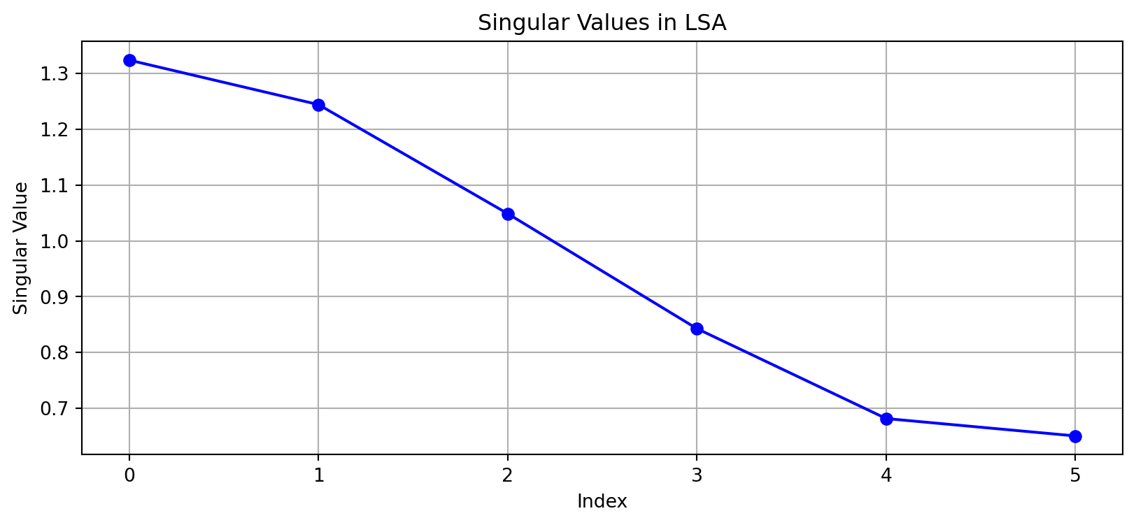
LSA typically uses a truncated SVD to reduce to \(k\) dimensions:
\[X_k = U_k\Sigma_k V_k^T\]
This reduction:
def plot_semantic_space(U, terms, k=2):
    # Project terms into semantic space
    term_coords = Vt[:k, :].T

    plt.figure(figsize=(12, 6))

    # Plot terms
    plt.scatter(term_coords[:, 0], term_coords[:, 1], c='blue', alpha=0.5)
    for i, term in enumerate(terms):
        plt.annotate(term, (term_coords[i, 0], term_coords[i, 1]))

    plt.title(f'{k}D Semantic Space')
    plt.xlabel('First Dimension')
    plt.ylabel('Second Dimension')
    plt.grid(True)
    plt.show()
    return

# Plot 2D semantic space
plot_semantic_space(U, terms)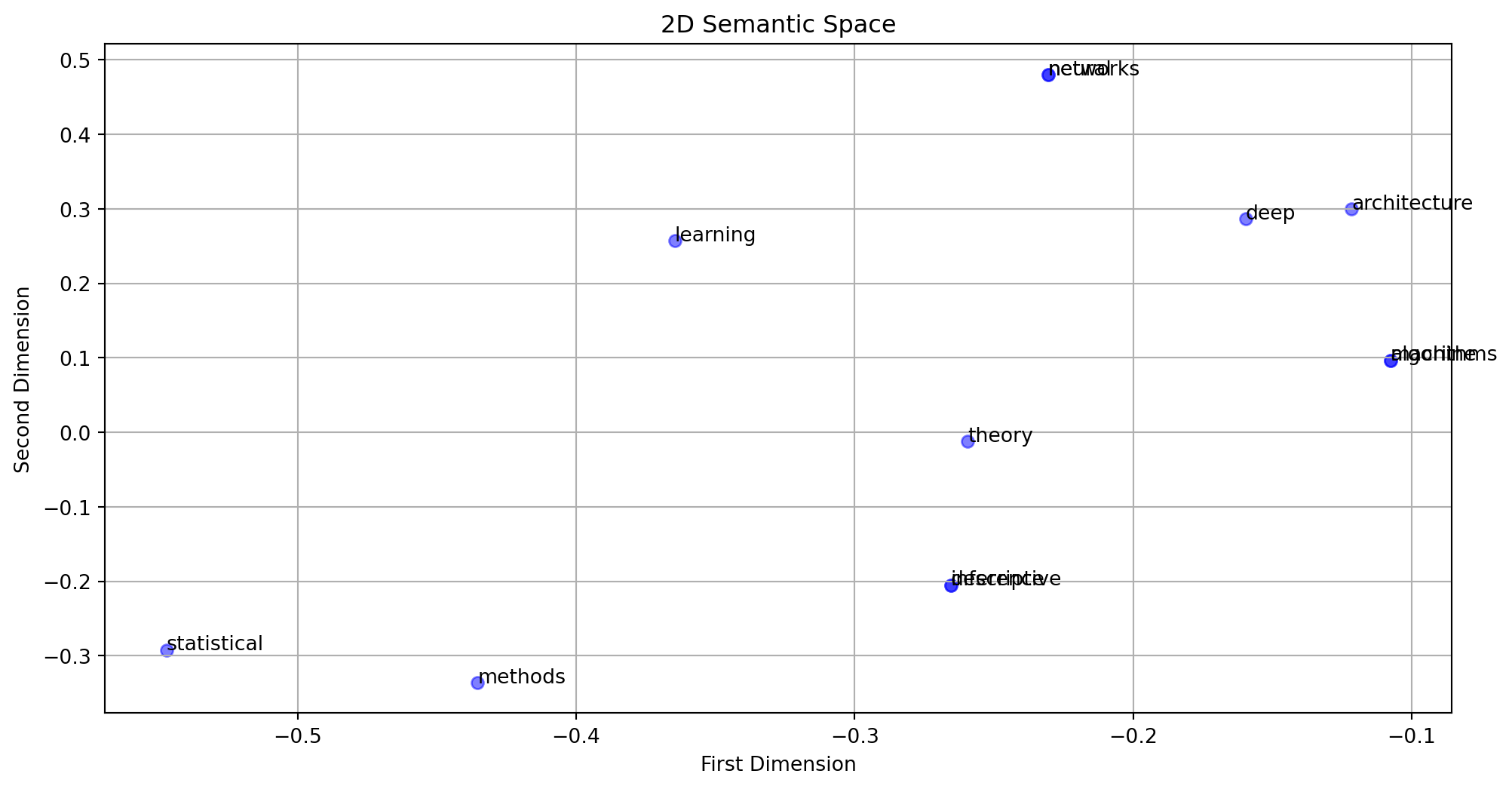
We can compute document similarity in the reduced space:
def compute_doc_similarity(X_reduced):
    # Normalize documents
    X_norm = normalize(X_reduced)
    # Compute cosine similarity
    similarity = X_norm @ X_norm.T
    return similarity

# Reduce to k dimensions
k = 2
X_k = U[:, :k] @ np.diag(s[:k]) @ Vt[:k, :]

# Compute and visualize similarities
sim_matrix = compute_doc_similarity(X_k)

plt.figure(figsize=(8, 6))
sns.heatmap(sim_matrix, annot=True, cmap='RdBu', center=0)
plt.title('Document Similarity Matrix')
plt.show()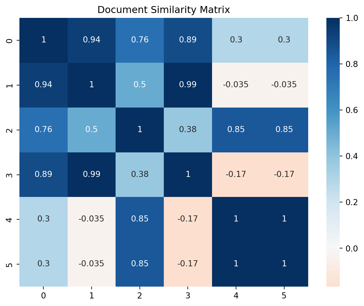
For a query vector \(q \in \mathbb{R}^p\), we project it into the LSA space:
\[q_k = q^T V_k \Sigma_k^{-1}\]
This gives us the query coordinates in the reduced concept space.
The similarity between query and documents is computed as:
\[\text{sim}(q, d_i) = \frac{q_k \cdot d_{ik}}{||q_k|| \cdot ||d_{ik}||}\]
where \(d_{ik}\) is the \(i\)-th row of \(D_k\).
def process_query(query, vectorizer, Vk, Sk, Dk, k):
    # Convert query to TF-IDF vector
    q = vectorizer.transform([query]).toarray()

    # Project query to LSA space
    qk = q @ Vk[:, :k] @ np.diag(1/Sk[:k])

    # Compute similarities
    similarities = np.dot(qk, Dk[:, :k].T)
    similarities = similarities / (np.linalg.norm(qk) *
                                np.linalg.norm(Dk[:, :k], axis=1))

    return similarities.flatten()

# Example query processing
k = 2  # number of dimensions to keep
Uk = U[:, :k]
Sk = s[:k]
Vk = Vt.T[:, :k]
Dk = Uk * Sk  # Document-concept matrix

query = "statistical"
similarities = process_query(query, vectorizer, Vt.T, s, Uk, k)

# Print results
for doc, sim in zip(corpus, similarities):
    print(f"Similarity: {sim:.3f} - {doc}")
Similarity: 0.346 - machine learning algorithms
Similarity: 0.019 - deep learning neural networks
Similarity: 0.890 - statistical learning theory
Similarity: -0.108 - neural networks architecture
Similarity: 0.994 - statistical inference methods
Similarity: 0.994 - statistical descriptive methodsThe LSA similarity measure has several important properties:
\[\text{sim}(t_i, t_j) = \frac{(V_k\Sigma_k)_i \cdot (V_k\Sigma_k)_j}{||(V_k\Sigma_k)_i|| \cdot ||(V_k\Sigma_k)_j||}\]
\[\text{context}(t_i) = \sum_{j \in \text{docs}} u_{jk}\sigma_k v_{ik}\]
The optimal number of dimensions \(k\) can be chosen based on:
\[\frac{\sum_{i=1}^k \sigma_i^2}{\sum_{i=1}^r \sigma_i^2} \geq \theta\]
\[\frac{\sigma_k - \sigma_{k+1}}{\sigma_k} \leq \epsilon\]
def plot_explained_variance(s):
    total_var = (s**2).sum()
    cum_var = np.cumsum(s**2) / total_var

    plt.figure(figsize=(8, 4))
    plt.plot(range(1, len(s) + 1), cum_var, 'b-o')
    plt.axhline(y=0.9, color='r', linestyle='--', label='90% threshold')
    plt.title("Cumulative Explained Variance")
    plt.xlabel("Number of components")
    plt.ylabel("Fraction of variance explained")
    plt.grid(True)
    plt.legend()
    plt.show()

plot_explained_variance(s)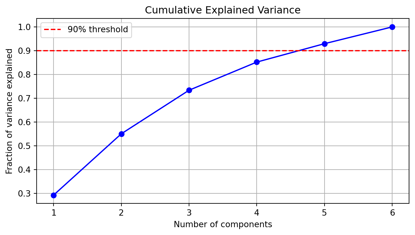
LSA can reveal term relationships through their positions in the semantic space:
from sklearn.cluster import KMeans

def plot_term_clusters(V, terms, k=2):

    # Use first k components
    term_coords = Vt[:k, :].T

    # Cluster terms
    kmeans = KMeans(n_clusters=3)
    kmeans.fit(term_coords)
    clusters = kmeans.predict(term_coords)

    plt.figure(figsize=(12, 6))
    scatter = plt.scatter(term_coords[:, 0], term_coords[:, 1],
                         c=clusters, cmap='viridis')

    for i, term in enumerate(terms):
        plt.annotate(term, (term_coords[i, 0], term_coords[i, 1]))

    plt.title('Term Clusters in Semantic Space')
    plt.colorbar(scatter)
    plt.show()

#plot_term_clusters(Vt, terms)LSA can be extended to multiple languages through parallel corpora:
The choice of dimensionality \(k\) depends on: 1. Corpus size and sparsity 2. Computational resources 3. Application requirements
def plot_explained_variance(s):
    var_explained = np.cumsum(s**2) / np.sum(s**2)

    plt.figure(figsize=(10, 4))
    plt.plot(var_explained, 'bo-')
    plt.axhline(y=0.9, color='r', linestyle='--')
    plt.title('Cumulative Explained Variance Ratio')
    plt.xlabel('Number of Components')
    plt.ylabel('Cumulative Explained Variance')
    plt.grid(True)
    plt.show()

plot_explained_variance(s)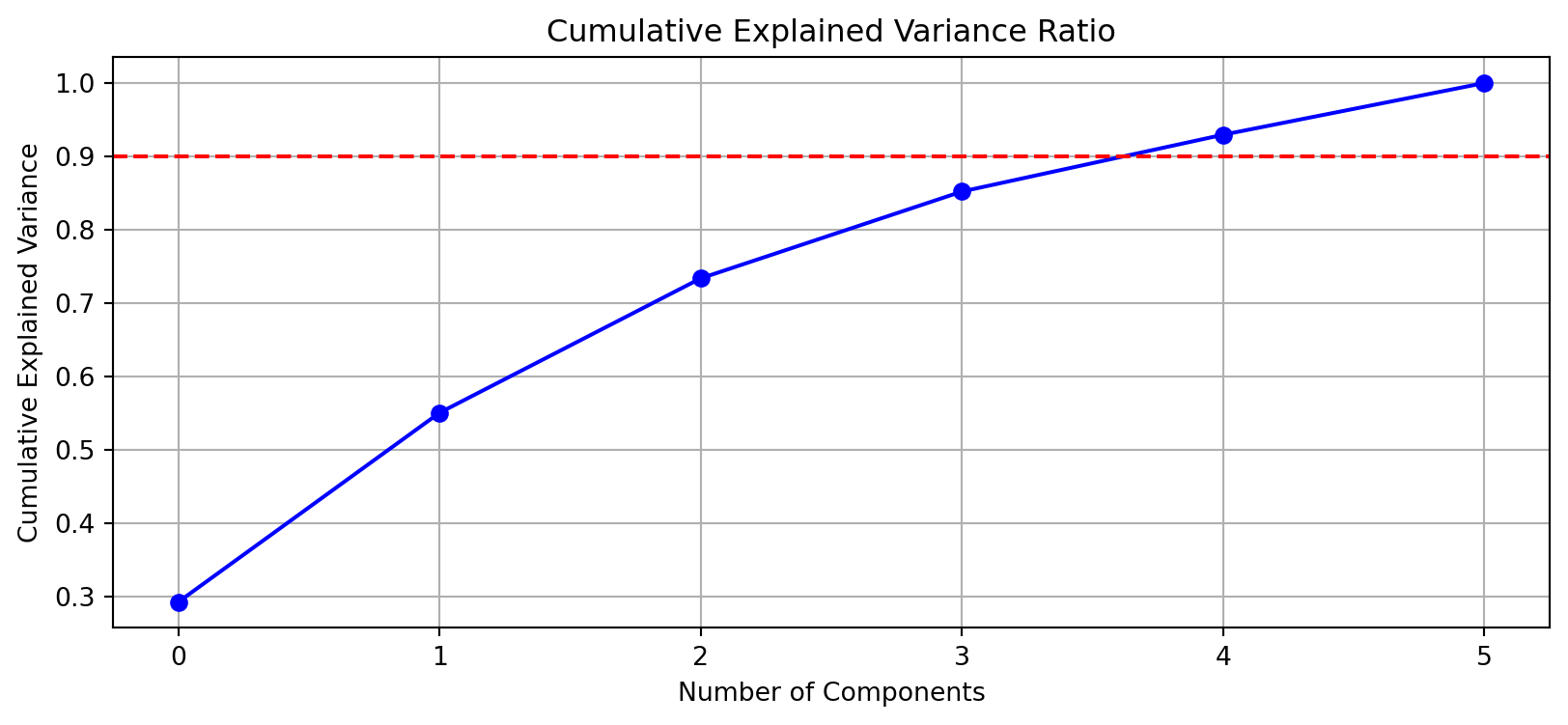
Text preprocessing significantly affects LSA results: - Stopword removal - Stemming/lemmatization - Case normalization - N-gram inclusion
Modern extensions include: - Probabilistic LSA (pLSA) - Latent Dirichlet Allocation (LDA) - Neural embeddings